MPI Finite Difference Phase Field Code - A Tutorial Guide

Table of Contents

Introduction
Understanding the Physics
MPI Concepts for Beginners
Step-by-Step Code Walkthrough
Visualization of Domain Decomposition
Communication Patterns Explained
Running the Code
Common Pitfalls and Solutions
Advanced Topics
Appendix: Quick Reference

Introduction

This document provides a comprehensive tutorial on parallel computing using MPI (Message Passing Interface) through a finite difference code that solves the Cahn-Hilliard equation—a fundamental model for phase separation in materials science. The code uses Eigen::Array for vectorized row access, float precision, and a load-balanced domain decomposition so the work divides evenly even when the grid size isn’t a multiple of the number of processes.

What You Will Learn

How to initialize and manage MPI processes
Load-balanced domain decomposition strategies for scientific computing
Communication patterns for finite difference stencils using Eigen row buffers
Data management with halo/ghost cells on Eigen::Array matrices
Performance optimization techniques (precomputed neighbor indices, -O3 -march=native, float precision)

Understanding the Physics

The Cahn-Hilliard equation describes phase separation in binary alloys:

\[\frac{\partial c}{\partial t} = \nabla \cdot \left[M \nabla \left(\frac{\delta F}{\delta c}\right)\right]\]

where:

\(c\): Concentration field
\(M\): Mobility
\(F\): Free energy functional

The code uses a 5-point finite difference stencil to discretize this equation spatially:

\[\nabla^2 c = \frac{c[i+1,j] + c[i-1,j] + c[i,j+1] + c[i,j-1] - 4c[i,j]}{\Delta x \cdot \Delta y}\]

Why Parallelize?

The 2D domain is \(5000 \times 5000\) grid points — 25 million points evolved for 1000 time steps.

Serial: 25 million points \(\times\) 1000 time steps = too slow on a single core.
Parallel: Domain divided among processors along the x-direction, each handling \(\sim 1/N\) of the rows, with remainder rows spread across the first few ranks so no process is left idle while others do extra work.

MPI Concepts for Beginners

What is MPI?

MPI is a standardized message-passing library designed for parallel computing. Think of it as a way for different computers (or processors) to talk to each other.

Key Concepts

Concept	Analogy	In Our Code
Rank	Worker ID number	Process identifier (0 to `size - 1`)
Communicator	Group of workers	`MPI_COMM_WORLD` (all processes)
Send/Recv	Passing notes	Exchanging boundary rows via `exchange_x_halos`
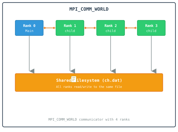
`MPI_PROC_NULL`	An empty mailbox	Used for the first/last rank’s missing neighbor, so no `if` branch is needed around the send/recv calls

Process Communication Model

Step-by-Step Code Walkthrough

Step 1: MPI Initialization

MPI_Init(&argc, &argv);

int rank, size;
MPI_Comm_rank(MPI_COMM_WORLD, &rank);
MPI_Comm_size(MPI_COMM_WORLD, &size);

if (rank == 0) {
    std::cout << "Total processors running: " << size << std::endl;
    std::cout << "Grid size: " << Nx << " x " << Ny << std::endl;
    std::cout << "Using float precision" << std::endl;
}

What happens here?

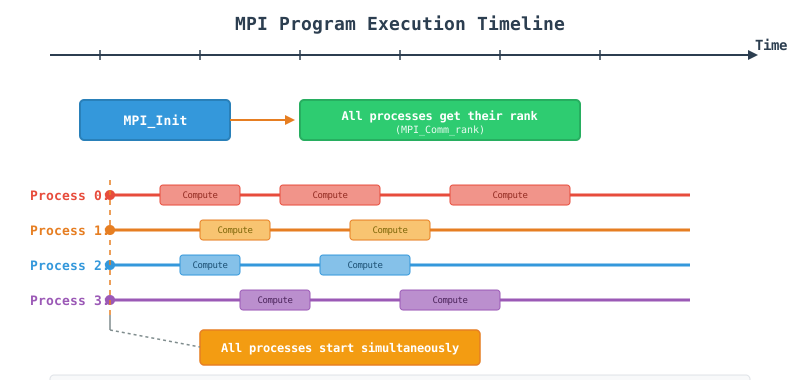
MPI_Init: Starts the MPI environment, sets up communication channels.
MPI_Comm_rank: Each process gets a unique ID (0 to size - 1).
MPI_Comm_size: Total number of processes running.
Only rank 0 prints the run configuration, so you don’t get the same three lines repeated once per process.

Visual Timeline:

Step 2: Load-Balanced Domain Decomposition

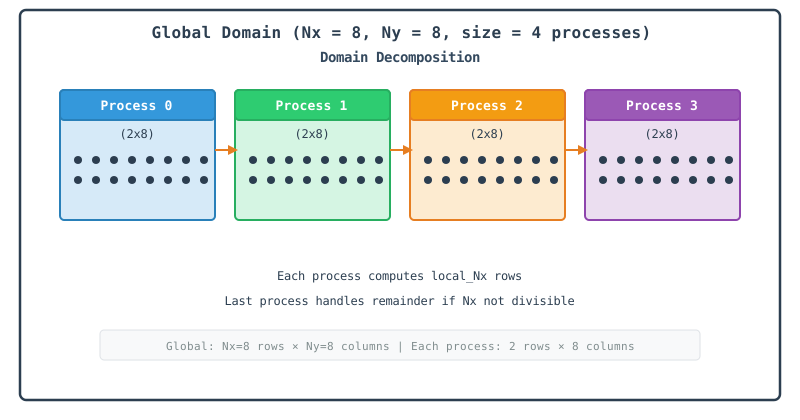
int base_Nx = Nx / size;
int remainder = Nx % size;

int local_Nx = base_Nx + (rank < remainder ? 1 : 0);
int start_x = rank * base_Nx + std::min(rank, remainder);
int end_x = start_x + local_Nx;

int local_Nx_halo = local_Nx + 2;

What happens here?

base_Nx: the guaranteed minimum number of rows every rank owns.
remainder: how many ranks need one extra row to cover the full domain.
local_Nx: ranks 0 through remainder - 1 get one extra row so the domain divides evenly overall.
start_x: computed with std::min(rank, remainder) so ranks after the first remainder ones are offset correctly once the extra rows run out.
local_Nx_halo = local_Nx + 2: two extra rows reserved for halo cells.

Visual Representation:

Step 3: Eigen-Based Halo Allocation

using EigenMatrix = Eigen::Array<float, Eigen::Dynamic, Eigen::Dynamic, Eigen::RowMajor>;

EigenMatrix con = EigenMatrix::Zero(local_Nx_halo, Ny);
EigenMatrix dfdcon = EigenMatrix::Zero(local_Nx_halo, Ny);
EigenMatrix lap_con = EigenMatrix::Zero(local_Nx_halo, Ny);
EigenMatrix dummy_con = EigenMatrix::Zero(local_Nx_halo, Ny);
EigenMatrix con_new = EigenMatrix::Zero(local_Nx_halo, Ny);

What happens here?

Eigen::Array<float, Dynamic, Dynamic, RowMajor> stores each row contiguously in memory, so a whole row can be sent with a single pointer and length in MPI_Sendrecv instead of looping element by element.
RowMajor is explicit here: Eigen defaults to column-major, which would make field.row(i).data() not point at contiguous memory.
EigenMatrix::Zero(...) allocates and zero-initializes in one call.
float precision keeps each array’s memory footprint and the bytes sent per halo exchange smaller — at \(5000 \times 5000\), each array is 100 MB.

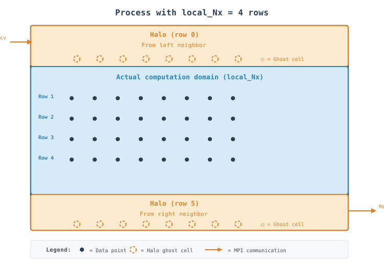
Halo Cells Visual:

Why are halos needed?

To compute derivatives at domain boundaries, we need values from adjacent rows.
Rank 1 needs a boundary row from rank 0 (left) and rank 2 (right).
Halos act as buffers that temporarily store these “ghost” values after communication.

Step 4: Data Initialization

std::mt19937 rng(rank + 12345);
std::uniform_real_distribution<float> dist(0.0f, 1.0f);

for (int i = 1; i <= local_Nx; ++i) {
    for (int j = 0; j < Ny; ++j) {
        con(i, j) = con_0 + noise * (0.5f - dist(rng));
    }
}

apply_periodic_y(con, local_Nx);

Important Points:

Each process initializes its own unique memory slice, using (row, col) Eigen accessors.
rank + 12345 ensures a unique random seed per process, preventing duplicate noise generation.
apply_periodic_y refreshes the y-boundary ghost columns right after initialization, since Eigen arrays have no built-in wraparound indexing.

Step 5: Communication - Halo Exchange as a Reusable Function

inline void exchange_x_halos(EigenMatrix& field, int local_Nx, int left, int right, 
                             MPI_Comm comm, MPI_Status& status) {
    // Send row 1 to left neighbor, receive into row local_Nx + 1 from right
    MPI_Sendrecv(field.row(1).data(), Ny, MPI_FLOAT, left, 0,
                 field.row(local_Nx + 1).data(), Ny, MPI_FLOAT, right, 0,
                 comm, &status);

    // Send row local_Nx to right neighbor, receive into row 0 from left
    MPI_Sendrecv(field.row(local_Nx).data(), Ny, MPI_FLOAT, right, 1,
                 field.row(0).data(), Ny, MPI_FLOAT, left, 1,
                 comm, &status);
}

What happens here?

field.row(1).data(): Eigen exposes a raw pointer into the row’s contiguous memory, so MPI_Sendrecv can be called exactly as it would be on a plain C array.
MPI_FLOAT matches the float precision of EigenMatrix.
left/right use MPI_PROC_NULL for the domain’s outer edges, so this function needs no special-casing for rank 0 or the last rank.
This function is reused for both con and dummy_con, since the stencil computation is split into two passes with a halo exchange between them.

Visual Communication Pattern:

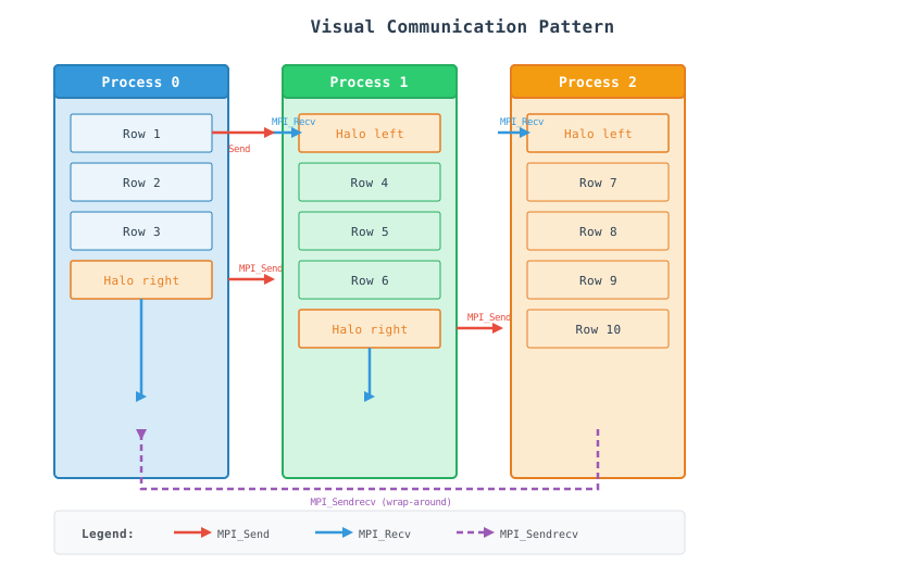
Step 6: Computation - Two Passes

Pass 1 — chemical potential:

inline void compute_laplacian_and_chemical_potential(
    const EigenMatrix& con, EigenMatrix& dfdcon, EigenMatrix& lap_con,
    EigenMatrix& dummy_con, int local_Nx,
    float dx, float dy, float A, float grad_coef)
{
    const float inv_dxdy = 1.0f / (dx * dy);

    static std::vector<int> jp(Ny), jm(Ny);
    static bool initialized = false;
    if (!initialized) {
        for (int j = 0; j < Ny; ++j) {
            jp[j] = (j + 1) % Ny;
            jm[j] = (j - 1 + Ny) % Ny;
        }
        initialized = true;
    }

    for (int i = 1; i <= local_Nx; ++i) {
        const auto& con_i = con.row(i);
        const auto& con_ip1 = con.row(i + 1);
        const auto& con_im1 = con.row(i - 1);
        auto dfdcon_i = dfdcon.row(i);
        auto lap_con_i = lap_con.row(i);
        auto dummy_con_i = dummy_con.row(i);

        for (int j = 0; j < Ny; ++j) {
            const float c = con_i(j);
            dfdcon_i(j) = A * (2.0f * c * (1.0f - c) * (1.0f - 2.0f * c));
            lap_con_i(j) = (con_ip1(j) + con_im1(j) +
                           con_i(jp[j]) + con_i(jm[j]) -
                           4.0f * c) * inv_dxdy;
            dummy_con_i(j) = dfdcon_i(j) - grad_coef * lap_con_i(j);
        }
    }
}

Pass 2 — second Laplacian and time integration:

inline void update_field(
    const EigenMatrix& con, const EigenMatrix& dummy_con, EigenMatrix& con_new,
    int local_Nx, float dt, float mobility, float inv_dxdy)
{
    static std::vector<int> jp(Ny), jm(Ny);
    // ... same precomputed neighbor tables ...

    const float factor = dt * mobility * inv_dxdy;

    for (int i = 1; i <= local_Nx; ++i) {
        const auto& con_i = con.row(i);
        const auto& dummy_i = dummy_con.row(i);
        const auto& dummy_ip1 = dummy_con.row(i + 1);
        const auto& dummy_im1 = dummy_con.row(i - 1);
        auto con_new_i = con_new.row(i);

        for (int j = 0; j < Ny; ++j) {
            const float lap_dummy = (dummy_ip1(j) + dummy_im1(j) +
                                    dummy_i(jp[j]) + dummy_i(jm[j]) -
                                    4.0f * dummy_i(j));
            float c_new = con_i(j) + factor * lap_dummy;
            con_new_i(j) = std::max(CLAMP_LOW, std::min(c_new, CLAMP_HIGH));
        }
    }
}

What happens here?

jp[j] / jm[j]: precomputed once via a function-local static array instead of recomputed with % on every inner-loop iteration.
con.row(i), con.row(i+1), etc. return Eigen expressions bound to const auto&, avoiding row copies while keeping the inner loop readable.
Pass 1 computes dfdcon, lap_con, and the chemical potential dummy_con.
Pass 2 computes lap_dummy from dummy_con’s neighbors and advances the concentration field with a clamped forward-Euler step: std::max(CLAMP_LOW, std::min(c_new, CLAMP_HIGH)).
dummy_con needs its own halo exchange (Step 7) before Pass 2 can read its neighboring rows correctly.

Step 7: The Evolution Loop

int left  = (rank == 0) ? MPI_PROC_NULL : rank - 1;
int right = (rank == size - 1) ? MPI_PROC_NULL : rank + 1;

for (int tsteps = 1; tsteps <= nsteps; ++tsteps) {
    exchange_x_halos(con, local_Nx, left, right, MPI_COMM_WORLD, status);

    compute_laplacian_and_chemical_potential(
        con, dfdcon, lap_con, dummy_con, local_Nx, dx, dy, A, grad_coef);

    exchange_x_halos(dummy_con, local_Nx, left, right, MPI_COMM_WORLD, status);

    update_field(con, dummy_con, con_new, local_Nx, dt, mobility, inv_dxdy);

    std::swap(con, con_new);
    apply_periodic_y(con, local_Nx);

    if (tsteps % nprint == 0 && rank == 0) {
        std::cout << "Done steps = " << tsteps << std::endl;
    }
}

What happens here?

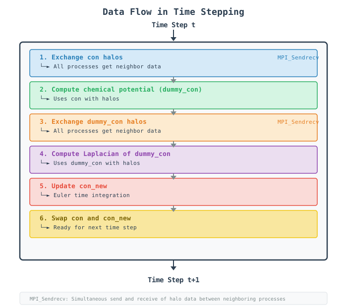
MPI_PROC_NULL makes MPI_Sendrecv treat the missing side as a no-op automatically, so exchange_x_halos needs no if (rank != 0) guard.
Each time step performs two halo exchanges: one for con before Pass 1, and one for dummy_con before Pass 2.
std::swap(con, con_new) is an O(1) pointer/metadata swap, no data copy.
apply_periodic_y(con, local_Nx) refreshes the ghost columns at j = 0 and j = Ny - 1 every step, right after the swap.

Data Flow in Time Stepping:

Step 8: Final Output

if (rank == 0) {
    std::cout << "  Total Run Time = " << (mpi_end_time - mpi_start_time) << " seconds." << std::endl;

    int rows_to_print = std::min(5, local_Nx);
    for (int i = 1; i <= rows_to_print; ++i) {
        for (int j = 0; j < 5; ++j) {
            std::cout << std::setw(10) << con(i, j) << " ";
        }
        std::cout << "\n";
    }

    int output_size = std::min(100, local_Nx);
    std::ofstream outfile("ch_small.dat");
    for (int i = 1; i <= output_size; ++i) {
        for (int j = 0; j < std::min(100, Ny); ++j) {
            outfile << con(i, j) << (j < 99 ? " " : "");
        }
        outfile << "\n";
    }
}

What happens here?

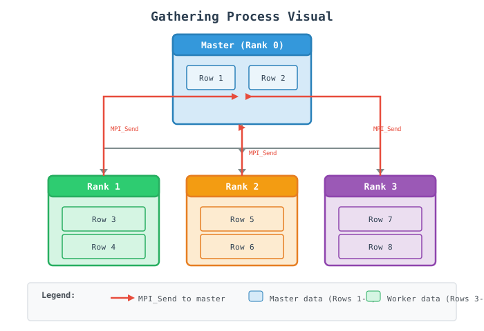
Only rank 0 prints and writes output — no gather step, so no communication happens in this stage.
rows_to_print: at most 5 rows, printed to the console for a quick sanity check.
output_size: up to a 100 x 100 corner of rank 0’s local con array, written to ch_small.dat.
All of the values printed and written here come from rank 0’s own local slice of the domain.

Gathering Process Visual:

Step 9: Timing and Performance Measurement

float mpi_start_time = MPI_Wtime();
// ... computation ...
float mpi_end_time = MPI_Wtime();

std::cout << "  Total Run Time = " << (mpi_end_time - mpi_start_time) << " seconds." << std::endl;

Wall-clock vs MPI Time:

Wall-clock time: Overall execution time including MPI overhead
MPI time:        Time spent in MPI operations (communication overhead)

Total Time = Computation Time + Communication Time + Idle Time

Visualization of Complete Communication Cycle

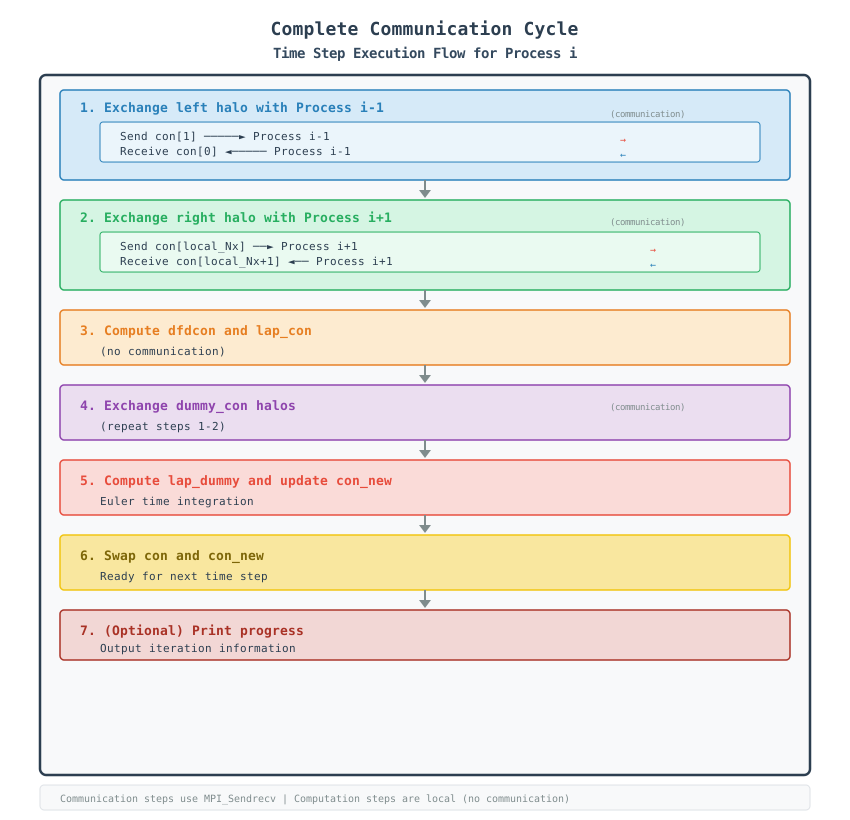
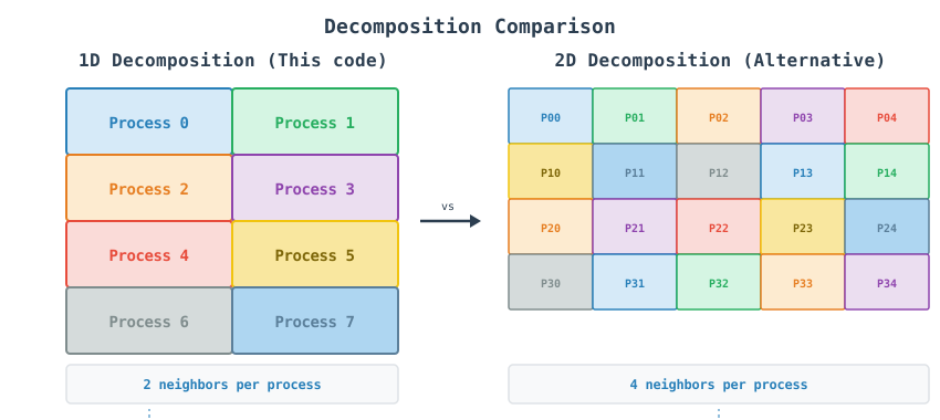
Why 1D Decomposition?

Advantages

Simple to implement with clear top/bottom boundary targets.
Only two active neighbors to manage (left and right).
Low code complexity for structured meshing.
Load-balanced across ranks (Step 2).

Disadvantages

Poor scalability ceiling if using thousands of ranks.
Network layout bottlenecks when partitioning data along only one direction.

Communication Patterns Explained

MPI_Sendrecv: The Superhero of MPI

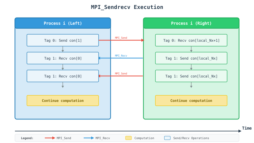
Why use MPI_Sendrecv instead of separate Send and Recv?

Problem with separate Send/Recv:

// DANGER: Potential Deadlock!
MPI_Send(field.row(1).data(), Ny, MPI_FLOAT, left, 0, MPI_COMM_WORLD);
MPI_Recv(field.row(local_Nx+1).data(), Ny, MPI_FLOAT, right, 0, MPI_COMM_WORLD, &status);

If both processes send first, both will wait forever (deadlock).

Solution with MPI_Sendrecv:

// SAFE: Combined send and receive handled safely by runtime engine
MPI_Sendrecv(field.row(1).data(), Ny, MPI_FLOAT, left, 0,
             field.row(local_Nx+1).data(), Ny, MPI_FLOAT, right, 0,
             MPI_COMM_WORLD, &status);

MPI handles the synchronization internally, preventing deadlocks. MPI_PROC_NULL means neither left nor right ever need to be checked before the call, since MPI silently skips the send or receive side when the partner is MPI_PROC_NULL.

Communication Timeline

MPI_Sendrecv Execution:

Blocking vs Non-blocking Communication

Aspect	Blocking (This code)	Non-blocking (Alternative)
Function	`MPI_Sendrecv` (via `exchange_x_halos`)	`MPI_Isend` / `MPI_Irecv`
Behavior	Waits for completion	Returns immediately
Overlap	No computation during communication	Can compute while communicating
Complexity	Simple	Requires `MPI_Wait` / `MPI_Test`
Performance	Lower for large messages	Higher potential performance

Non-blocking would look like:

MPI_Request req[4];
MPI_Isend(field.row(1).data(), Ny, MPI_FLOAT, left, 0, MPI_COMM_WORLD, &req[0]);
MPI_Irecv(field.row(local_Nx + 1).data(), Ny, MPI_FLOAT, right, 0, MPI_COMM_WORLD, &req[1]);
// Compute here while communication happens!
MPI_Waitall(2, req, MPI_STATUSES_IGNORE);

Running the Code

Compilation

Linux (GCC/OpenMPI, with Eigen headers on the include path):

mpic++ main.cpp -O3 -march=native -std=c++20 -I /usr/include/eigen3/ -o main

Windows (Intel MPI):

mpiicpx -I"C:\libs\eigen-5.0.0" main.cpp

Eigen is a header-only library, so -I points at the headers and nothing needs to be linked. -march=native lets the compiler auto-vectorize the float stencil loops for the specific CPU it’s built on.

Running

Basic Run (4 processes):

mpirun -np 4 ./main

Scale -np based on available cores and memory — each rank needs local_Nx_halo x Ny x 4 bytes x 5 arrays of memory.

Common Pitfalls and Solutions

1. Column-Major Eigen Arrays

Problem:

// Wrong: default Eigen storage order is ColMajor
using EigenMatrix = Eigen::Array<float, Eigen::Dynamic, Eigen::Dynamic>;
// field.row(i).data() no longer points at contiguous row memory!

Solution:

// Correct: explicit RowMajor storage
using EigenMatrix = Eigen::Array<float, Eigen::Dynamic, Eigen::Dynamic, Eigen::RowMajor>;

field.row(i).data() must point to Ny contiguous floats for MPI_Sendrecv to work correctly.

2. Forgetting the Second Halo Exchange

Problem:

exchange_x_halos(con, local_Nx, left, right, MPI_COMM_WORLD, status);
compute_laplacian_and_chemical_potential(con, dfdcon, lap_con, dummy_con, ...);
// Missing: exchange_x_halos(dummy_con, ...)
update_field(con, dummy_con, con_new, ...);  // reads stale dummy_con halos!

Solution: Exchange dummy_con’s halos between the two computation passes, as shown in Step 7.

3. Forgetting `apply_periodic_y` After the Swap

Problem:

std::swap(con, con_new);
// Missing: apply_periodic_y(con, local_Nx);
// Next iteration's stencil reads stale y-boundary values from before the swap

Solution: Call apply_periodic_y(con, local_Nx) immediately after every swap, as shown in Step 7.

4. Mismatched MPI Datatype

Problem:

MPI_Sendrecv(field.row(1).data(), Ny, MPI_DOUBLE, left, 0, ...);  // Wrong! Array is float

Solution:

MPI_Sendrecv(field.row(1).data(), Ny, MPI_FLOAT, left, 0, ...);  // Matches EigenMatrix's float

5. Assuming Rank 0’s Output Is the Full Domain

Problem: Treating ch_small.dat as a full-field snapshot, when it only contains rank 0’s local corner.

Solution: Add a gather step (see Advanced Topics) if the complete 5000 x 5000 field is needed.

Advanced Topics

Full-Domain Gather

To collect the complete field on rank 0 (e.g. for plotting):

if (rank == 0) {
    EigenMatrix full_con = EigenMatrix::Zero(Nx, Ny);
    full_con.block(start_x, 0, local_Nx, Ny) = con.block(1, 0, local_Nx, Ny);

    for (int p = 1; p < size; ++p) {
        int p_local_Nx = base_Nx + (p < remainder ? 1 : 0);
        int p_start_x  = p * base_Nx + std::min(p, remainder);

        std::vector<float> recv_buf(p_local_Nx * Ny);
        MPI_Recv(recv_buf.data(), p_local_Nx * Ny, MPI_FLOAT, p, 0,
                 MPI_COMM_WORLD, MPI_STATUS_IGNORE);
        // Copy recv_buf into full_con.block(p_start_x, 0, p_local_Nx, Ny)
    }
} else {
    MPI_Send(con.data() + Ny, local_Nx * Ny, MPI_FLOAT, 0, 0, MPI_COMM_WORLD);
}

Each rank’s row count and starting offset are recomputed with base_Nx / remainder, since the decomposition is load-balanced rather than uniform.

Non-blocking Halo Exchange

Convert exchange_x_halos to MPI_Isend/MPI_Irecv so the CPU can start compute_laplacian_and_chemical_potential on interior rows while boundary rows are still in flight.

MPI + OpenMP Hybrid

Combine with OpenMP to parallelize the inner j loops of compute_laplacian_and_chemical_potential and update_field within each rank:

#pragma omp parallel for
for (int i = 1; i <= local_Nx; ++i) {
    // existing row-wise computation
}

Precision Trade-offs

float halves memory and communication volume relative to double, at the cost of reduced precision — worth profiling both for simulations sensitive to numerical drift over long runs.

Appendix: Quick Reference

Key Constants

Constant	Value
`Nx`, `Ny`	5000, 5000
`nsteps`	1000
`dt`	0.01f
Precision	`float`
`CLAMP_LOW` / `CLAMP_HIGH`	`1e-5f` / `0.99999f`

MPI Functions Used

Function	Purpose
`MPI_Init` / `MPI_Finalize`	Start/stop the MPI environment
`MPI_Comm_rank` / `MPI_Comm_size`	Identify this process / count all processes
`MPI_Sendrecv`	Combined, deadlock-safe send + receive
`MPI_PROC_NULL`	“No-op” neighbor for domain edges
`MPI_Wtime`	High-resolution wall-clock timer

Eigen Types Used

Type	Purpose
`Eigen::Array<float, Dynamic, Dynamic, RowMajor>`	The `EigenMatrix` alias — contiguous rows for MPI
`EigenMatrix::Zero(rows, cols)`	Allocate + zero-initialize
`field.row(i)`	Row accessor, `.data()` gives a raw contiguous pointer
`field.block(row, col, rows, cols)`	Sub-block view/assignment, useful for gather-style code

MPI Finite Difference Phase Field Code - A Tutorial Guide

Table of Contents

Introduction

What You Will Learn

Understanding the Physics

Why Parallelize?

MPI Concepts for Beginners

What is MPI?

Key Concepts

Process Communication Model

Step-by-Step Code Walkthrough

Step 1: MPI Initialization

What happens here?

Visual Timeline:

Step 2: Load-Balanced Domain Decomposition

What happens here?

Visual Representation:

Step 3: Eigen-Based Halo Allocation

What happens here?

Halo Cells Visual:

Why are halos needed?

Step 4: Data Initialization

Important Points:

Step 5: Communication - Halo Exchange as a Reusable Function

What happens here?

Visual Communication Pattern:

Step 6: Computation - Two Passes

What happens here?

Step 7: The Evolution Loop

What happens here?

Data Flow in Time Stepping:

Step 8: Final Output

What happens here?

Gathering Process Visual:

Step 9: Timing and Performance Measurement

Wall-clock vs MPI Time:

Visualization of Complete Communication Cycle

Why 1D Decomposition?

Advantages

Disadvantages

Communication Patterns Explained

MPI_Sendrecv: The Superhero of MPI

Why use MPI_Sendrecv instead of separate Send and Recv?

Problem with separate Send/Recv:

Solution with MPI_Sendrecv:

Communication Timeline

MPI_Sendrecv Execution:

Blocking vs Non-blocking Communication

Non-blocking would look like:

Running the Code

Compilation

Running

Common Pitfalls and Solutions

1. Column-Major Eigen Arrays

2. Forgetting the Second Halo Exchange

3. Forgetting apply_periodic_y After the Swap

4. Mismatched MPI Datatype

5. Assuming Rank 0’s Output Is the Full Domain

Advanced Topics

Full-Domain Gather

Non-blocking Halo Exchange

MPI + OpenMP Hybrid

Precision Trade-offs

Appendix: Quick Reference

Key Constants

MPI Functions Used

Eigen Types Used

3. Forgetting `apply_periodic_y` After the Swap